While AGI may still be a few decades in the horizon, researchers have long been trying to mimic the human brain. Just like its namesake, the neural network works in the same way a neuron in the human body does. It receives stimuli, processes it and sends stimuli to the next neuron.
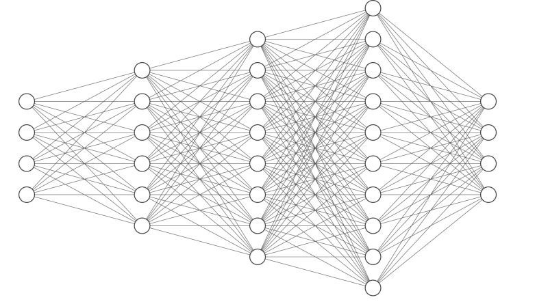
This is achieved using layers- input, output and various hidden layers. Each layer has a varying number of units, depending on the amount of data to be processed and the nature of the data. Each layer has a specific activation function it uses to process the data.
This function exists to ensure that processing is not restricted to learning linear relationships, which means that the network is capable of learning complex, non-linear patterns in data. It also regulates how signals propagate through the network, compress and normalise signals (e.g., sigmoid) or allow them to pass largely unchanged and mitigate issues like vanishing or exploding gradients.
It is these activation functions which help us achieve something close to the firing patterns of neurons in biological brains. This makes the right selection of an activation function of a layer extremely important, contributing largely to learning speed, computational efficiency, and the network’s ability to model complex relationships.
The choice of activation function can mean the difference between a model that learns effectively and one that struggles with issues like vanishing gradients or slow convergence. As neural network architectures have evolved, so too has our understanding of activation functions and their impact on model performance. This evolution has led to the development of various types of activation functions, each with its own characteristics and strengths.
Sigmoid:
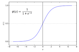
Function: f(x) = 1 / (1 + e^(-x))
The sigmoid function compresses the input values to the range (0, 1). It makes the data smooth and continuously differentiable. Historically popular, it’s now mainly used in the output layer for binary classification problems. The function saturates and kills gradients for very high or very low input values, which can slow down or halt learning in deep networks (vanishing gradient problem).
Softmax:
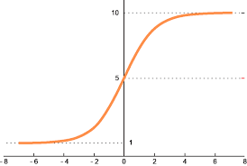
Function: f(x_i) = e^(x_i) / Σ(e^(x_j))
Softmax is typically used in the output layer for multi-class classification problems. It converts a vector of real numbers into a probability distribution, where the probabilities sum to 1. This makes it easy to interpret the network’s output as class probabilities. It’s computationally more expensive than other activation functions, especially for a large number of classes. However, it is one of the more diverse activation functions typically used for probabilistic predictions, NLPs and Reinforcement Learning.
Rectified Linear Unit (ReLU):
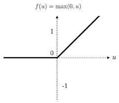
Function: f(x) = max(0, x)
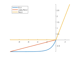
ReLU is computationally efficient and helps alleviate the vanishing gradient problem. This is the activation function most commonly used for hidden layers. It allows for sparse activation in neural networks, as it sets all negative inputs to zero. This sparsity can be beneficial for computational efficiency and representation learning. However, ReLU can suffer from the “dying ReLU” problem, where neurons can get stuck in an inactive state if they consistently receive negative inputs.
Leaky ReLU:
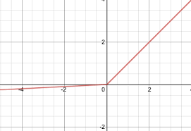
Function: f(x) = x if x > 0, else αx (where α is a small constant, typically 0.01)
Leaky ReLU addresses the dying ReLU problem by allowing a small gradient when the unit is not active. This helps prevent neurons from getting stuck in an inactive state. The small slope for negative inputs allows for some information to flow even when the neuron is not strongly activated, leading to more effective learning in deep networks. It doesn’t completely discard negative inputs thus beneficial for tasks where negative signals are important. While still promoting some sparsity, it’s less extreme than ReLU, it maintains most of ReLU’s computational benefits and only slightly more complex than standard ReLU.
Exponential Linear Unit (ELU) and SELU:
Function: f(x) = x if x > 0, else α(e^x – 1) (where α is typically 1)
ELU combines the benefits of ReLU (addressing vanishing gradients) with the ability to produce negative outputs unlike ReLU. The smooth function near zero helps in reducing the bias shift that ReLU can suffer from, helping in more robust learning and potentially better gradients. ELUs push mean activations closer to zero, which can help with internal covariate shift. ELU can result in faster learning and better generalization, but it’s computationally more expensive than ReLU.
Linear:
Function: f(x) = x
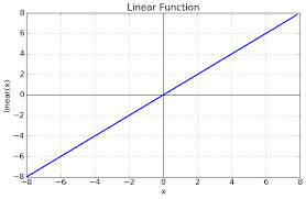
The linear activation function is simply the identity function. The output is directly proportional to the input, which can be desirable in some cases. It needs no complex calculations, making it fast to compute and easy to use in conjunction with non-linear activations in other layers. It’s typically used in the output layer for regression problems and isolate issues in network architecture or data preprocessing. While it doesn’t add non-linearity to the network, it’s useful when you want the network to output unbounded values.
Swish:
Function: f(x) = x * sigmoid(βx) (where β is a learnable parameter or set to 1)
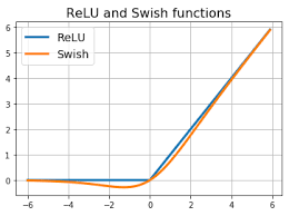
Swish is a relatively new activation function that has shown promising results in deep networks. It’s smooth, non-monotonic, and unbounded above. The shape of the Swish function allows it to carry some small negative values, which can be beneficial for learning. Swish has a lower bound, which can help prevent exploding gradients in deep networks. It often outperforms ReLU in deep networks and also mitigate the bias shift problem that ReLU sometimes encounters but is computationally more expensive.
Each function has its strengths and weaknesses. Sigmoid and tanh, while useful for specific tasks, can suffer from vanishing gradients. ReLU and its variants (Leaky ReLU, PReLU) have become popular due to their simplicity and effectiveness in mitigating gradient issues, though they may face problems like dying, inactive neurons. ELU and SELU aim to combine ReLU’s benefits with improved handling of negative inputs, at the cost of increased computational complexity. Swish has shown promising results in deep networks but is also more computationally intensive than ReLU.
The choice of activation function depends on the specific task, network architecture, and computational constraints. ReLU and its variants are often good default choices for hidden layers due to their simplicity and effectiveness. Sigmoid and softmax remain crucial for binary and multi-class classification output layers, respectively. For regression tasks, linear activation in the output layer is common.
As research continues, new activation functions keep emerging, potentially offering improved performance or addressing specific challenges. The key is to understand the properties of each function and how they align with the requirements of your particular neural network application.
Ultimately, the selection of activation functions often involves empirical testing and consideration of trade-offs between performance, computational efficiency, and the specific demands of the problem at hand. As with many aspects of deep learning, there’s no one-size-fits-all solution, and the optimal choice may vary depending on the unique characteristics of each task and dataset.
Be First to Comment